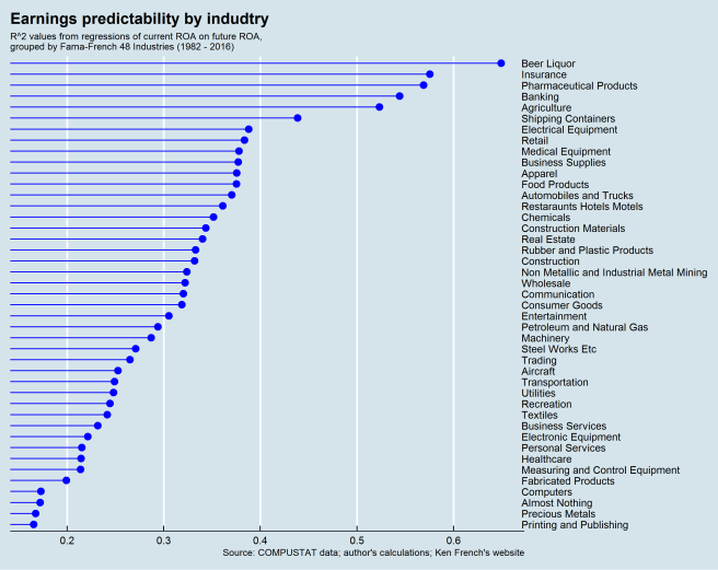
How well does the AR(1) model of earnings predict in-sample and out-of-sample?
To answer this question I take the simple first-order autoregressive model, ,
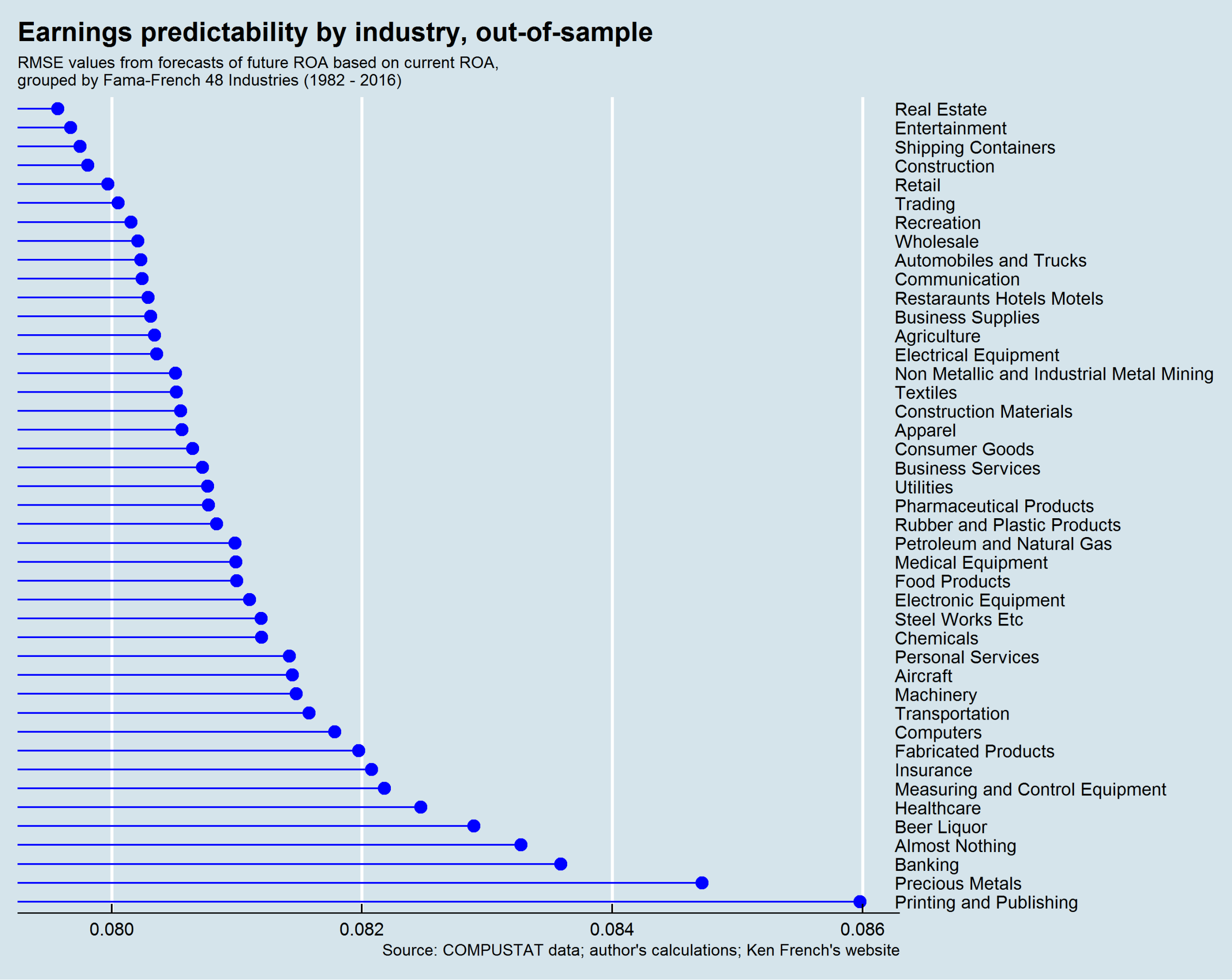
evaluate it on a 60/40 training/test set of firm earnings, and calculate it’s (training sample) and (test set) root-mean-square prediction error.
By the top five industries are Beer and Liquor, Insurance, Pharmaceuticals, Banking, and Agriculture.
Based on RMSE, the most predictable industries are Real Estate, Entertainment, Shipping Containers, Construction, and Retail.
Based on both and RMSE, the only industry to be in the top ten for both metrics is Retail.
In this post I will describe a method for downloading a large number of files from the internet using Amazon Web Services (AWS). This is useful if you have lots of files to download, but you don’t want to tie up your own machine for days and/or you don’t have the hard drive space for the files. This is one solution to this problem, I’m sure there are many others.
This post is a prelude to a future post on quickly downloading company filings from the SEC’s EDGAR server. However, the method described is more general. It can be applied to the bulk distributed downloading of any type of data.
Development Environment
The pieces of AWS infrastructure we’ll be using are EC2 and S3. Amazon provides detailed and up-to-date instructions for setting up an AWS development environment. Use theirs.
All code is in Python 2 on Linux (Ubuntu). You will need to set-up the AWS command-line interface (awscli) for use on your local machine. You will need the Amazon Python SDK, Boto3.
I will create an EC2 instance with Ubuntu, install the dependencies, and clone the instance as an Amazon Machine Image (AMI). Once the instance image is created, we can clone our remote development environment and execute code on multiple separate but identical EC2 instances.
Programming Model
Get a list of URLs you want to download
Spin up n EC2 instances
Split the list of URLs into n equal-sized chunks.
Execute script to download URLs on each EC2 instance.
Execute script to send downloaded files from each EC2 instance to S3.
Data Location
Local Machine: A Python driver for the remote python script; list of URLs. Remote EC2 Instance: Sample list of URLs. S3 Bucket: Downloaded files.
Implementation
To illustrate, let’s download all 5,293 zip files containing server log data for the SEC. You can read more about the data on the SEC’s website here.
Create an EC2 instance with Ubuntu. Install the necessary software dependencies.
1. Download the list of zip files from EDGAR.
sec_logfile_data_url = "https://www.sec.gov/files/EDGAR_LogFileData_thru_Jun2017.html"

## Read in LogFile list from EDGAR
sec_zipfile_list = urllib.urlretrieve(sec_logfile_data_url, "logfilelist.html")

## Generate list of log file ZIP files
sec_zipfile_list = open("logfilelist.html", "r").readlines()
sec_zipfile_list = [x.strip() for x in sec_zipfile_list]
## skip first few lines (html header data)
sec_zipfile_list = sec_zipfile_list[9:]

with open("logfile-urls.txt", "w") as outfile:
    outfile.writelines([x+'\n' for x in sec_zipfile_list])
As the code shows, the list of URLs for the zip files containing the SEC server logs will be stored in a file “logfile-urls.txt”.
2. Initiate Remote EC2 Instances
Next, spin up the EC2 instances and store the associated IP addresses in a list. In the code below AMI_ID is your Amazon Machine Image ID, the AMI code of your cloned EC2 instance and SEC_GROUP_ID is the name of your AWS security group for this AMI. I’ve chosen to create up to 20 instances (MaxCount = 20) of t2.medium CPU types. Read more about Amazon EC2 instance types here. The “t2.medium” type will be fine for our purposes.
After the instances have finished starting up (you can check via the EC2 console), store their IPs:
ec2 = boto3.resource('ec2')
instances = ec2.instances.filter(Filters=[{'Name': 'instance-state-name', 'Values': ['running']}])
ec2_instance_list = [i.public_ip_address for i in instances]
3. Distribute URLs to Download
Split the list of URLs into 10 different chunks, one for each EC2 instance we will create. Locally, each sample of URLs that will be distributed will have a filename of the form url-IP.ADRESS, where the “IP.ADDRESS” field is the IP address of the remorte EC2 instance where the files will be distributed and downloaded. On the instances themselves, this file will be named simply “urls.txt”. Note below the variable PEM_KEY_LOC–since we are using scp to download the files, you will need to tell the AWS command-line interface where your .pem key file is located and set it here.
def send_urls_helper(start_index, stop_index, ec2_IP):
    ## create file name for sample of URLs to be sent to this EC2 instance
    urls_sample_filename = "urls-%s.txt" % ec2_IP

    ## Get sample of URLs to send to this EC2 instance
    urls = open(_URLS,'r').readlines()
    urls = urls[start_index:stop_index]
    with open(urls_sample_filename,'w') as outfile:
        outfile.writelines(urls)

    ## Send URLs file to EC2 instance
    os_command = "scp -o StrictHostKeyChecking=no -i %s %s ubuntu@%s:urls.txt" % (PEM_KEY_LOC, urls_sample_filename, ec2_IP)
    print os.system(os_command), os_command
    return None

## Split large URLs file into equal-sized chunks and send to each EC2 instance
def send_urls(ec2_instance_list=[], urls_location=""):
    n_instances = len(ec2_instance_list)
    urls = open(urls_location,'r').readlines()
    n_files = len(urls)
    sample_size = n_files/n_instances
    print '%d files, %d instances, %d files per instance' % (n_files, n_instances, sample_size)
    i = 0
    while i < (n_instances-1):
        send_urls_helper(i*sample_size, (1+i)*(sample_size), ec2_instance_list[i])
        i += 1
    if i == (n_instances-1):
        send_urls_helper(i*sample_size, n_files, ec2_instance_list[i])
    return None
4. Download
Using a combination of Linux’s wget (for downloading from the internet) and xargs (for multithreading), the code below sends a command to each EC2 instance to download its URLs.
The zip files will download on each EC2 instance. After they are finished, the last step is to collect them for extracting (untar and unzip) and analyzing (for “doing science” on). The two most straight-forward methods are (1) using scp to copy the files to your local machine; and (2) transferring the files to an Amazon S3 bucket. The code below does the latter.
In this post and the next, I build up to a VAR analysis in R–exploring the dynamics of aggregate net income, cash flow, and accruals and returns. Aggregate time series analysis is becoming very popular in accounting research. I want to provide a quick look at getting started in R on the different steps in a time series analysis on data familiar to researchers in accounting and finance.
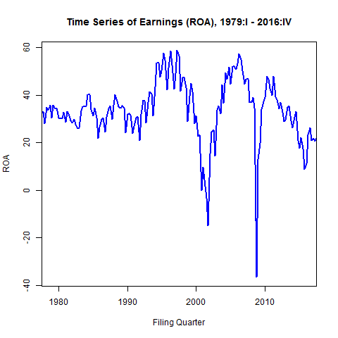
I will model raw quarterly net income (un-weighted, not scaled by, e.g., assets) from 1961 – 2017 for firms in COMPUSTAT. I’ve applied some basic filters for size, liquidity, and operating activity. For forecasting purposes, I will split the sample into training and test samples. The test sample will be the last two years (8 quarters of observations).
I decompose the trend, seasonal, and cyclical components of earnings using the stl() command. The stl() function assumes an additive series structure: . Where S, T, and E refer to the seasonal, trend, and residual (error) components, respectively.
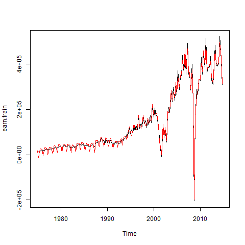
Using the seasonadj() function in forecast, I can plot the seasonally-adjusted earnings series (in red). For much of the sample period there doesn’t seem to be a significant seasonal pattern to the data. I could do a lot more to examine potential seasonality of the data, but I’ll ignore it for now.
Are Earnings Stationary?
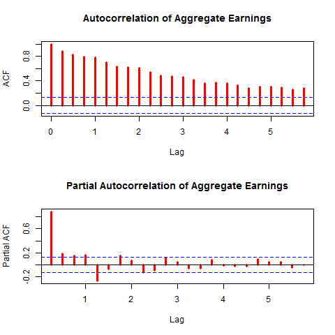
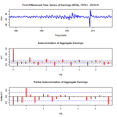
Nonstationary time series can lead to poor inferences in modeling, specifically spurious regressions[1] and poor forecasting performance. If variables are nonstationary we can often use a simple transformation, such as first-differencing the series or taking log transformations, to make them stationary. From the plot of aggregate earnings above, it doesn’t seem likely that earnings are stationary. As another way explore the autocovariance structure graphically I show autocorrelation and partial autocorrelation function graphs below.
Note the slow decay in the ACF graph and the lags that are statistically significant correlates with earnings shown in the PACF. This is more evidence that the series is not stationary. Formally I perform Augmented Dickey-Fuller (ADF) tests on the series to test the null hypothesis of nonstationarity.
ADF Test
The Dickey-Fuller test for stationarity is based on an AR(1) process:
where
or, in the case of a series displaying a constant and trend
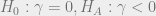
According to the Dickey-Fuller test, a time series is nonstationary when , which makes the AR(1) process a random walk. The null and alternative hypotheses of the test are
The basic AR(1) equations mentioned above are transformed, for the purpose of the DF test into
with the transformed hypothesis as
The Augmented DF test includes several lags of the variable tested. The ADF test can be of three types: with no constant and no trend, with constant and no trend, and, finally, with constant and trend. It is important to specify which DF test we want because the critical values are different for the three different types of the test. The R function adf.test() in the tseries package tests for a constant and a linear trend.[2] Our time series is stationary if we are able to reject the null hypothesis of the ADF test.
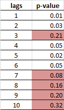
There has been a lot of work on selecting the optimal lag length in ADF tests (see for examples [3] and [4]). In R I will investigate the tests for one to 10 lags.
k <- 10
X <- data.frame(matrix(NA, nrow = k, ncol = 2))
names(X) <- c('lags', 'p-value')
X[, 'lags'] <- 1:k
for(i in 1:k) X[i, 'p-value'] <- tseries::adf.test(earnings$roa, k = i)$p.value
The results fail to reject the null of nonstationarity in every case, as expected. However, a simple first differencing of earnings leads to a stationary series. This implies the series is of order one integration I(1). The figures below show the time series, ACF, and PACF plots of the first-differenced earnings series. The ADF test for lags one through ten all reject the null of nonstationarity. This will be useful later for forecasting.
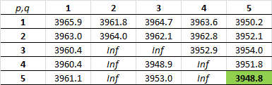
We will train a model on the differenced data. For forecasting, I’ll consider all possible ARMA(p,q) models with . The auto.arima() function in the forecast package does this nicely. The best model based on AIC is of ARMA(5,5).
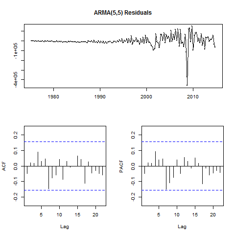
I’ll next examine the residuals of the model I’ve developed on the training data, prior to forecasting on the test data. The residuals() function combined with tsdisplay() from the forecast package will plot these diagnostics.
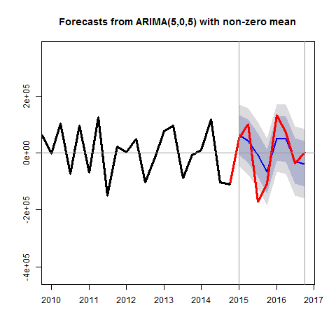
The figure below shows the forecast generated from this model in the last eight quarters of the sample (the hold-out sample). I’ve included error bands and superimposed the actual realizations.
It’s important to keep in mind that what we’ve forecasted here is the change in earnings. The next step in implementing this model in a forecasting scenario might be to convert the model for the differenced earning series to one for the levels.
References: [1] Hilarious examples abound here: http://www.tylervigen.com/spurious-correlations. Most, if not all, of these correlations would go away if the series in question were first-differenced.
[2] There are various implementations of the ADF test in R, all of differing degrees of confusing, which I will cover in a future post.
[3] Ng and Perron “Unit Root Tests in ARMA Models with Data-Dependent Methods for the Selection of the Truncation Lag,” JASA, 1995.
[4] Schwert, GW “Tests for Unit Roots – A Monte-Carlo Investigation,” Journal of Business & Economic Statistics, Apr 1989. Vol 7. Issue 2. Pages 147-159.
There are a lot of great data science initiatives going on at campuses right now. I had the pleasure of attending a symposium at the University of Michigan recently. It was a great way to learn about data science going on in academia across departments. The folks at the Michigan Institute for Data Science (MIDAS) have been kind enough to post the videos from the forum on YouTube. Definitely check them out here!
Of particular interest for researchers in applied social sciences like mine (finance and accounting) is the session on partnering with industry: here.
A common task in preparing data for analysis is to Winsorize variables in the dataset first. This means we want to replace extreme values in the data with less extreme values. This is usually operationalized as replacing values of a variable, say return on assets (ROA), that are above the 99th percentile with the 99th percentile value itself, and ROA values below the 1st percentile with the 1st percentile value itself. It is a form of outlier reduction. See the Wikipedia article.
In R, for a single variable we can do this in a few lines integrating the quantile function:
wins <- function(x){
  ## A helper function for wins.df
  ## x: is a vector
  percentiles <- quantile(x, probs=seq(0,1,0.01), na.rm=TRUE)
  pLOWER <- percentiles["1%"]
  pUPPER <- percentiles["99%"]
  x.w <- ifelse(x <= pLOWER, pLOWER, x)
  x.w <- ifelse(x >= pUPPER, pUPPER, x.w)
  return(x.w)
}
In a pooled cross-section of data, we usually want to Winsorize at the yearly frequency. Passing the above wins function as a helper to a larger one this can be extended pretty straightforwardly:
wins.df <- function(X, var, yearid = "year"){
  years <- unique(X[,yearid])
  Y <- X
  for(year in years){
    x <- X[which(X[, yearid] == year), var]
    x.w <- wins(x)
    var.w <- var
    Y[which(Y[,yearid] == year), var.w] <- x.w
  }
  return(Y)
}
A cleaned-up and more general version of this code is here.
This is the first part in a series of posts that cover how to download and analyze SEC filings. In this post I will show how to retrieve the URLs for the filings you want from the SEC server. Most advice floating around today involves using the now discontinued SEC ftp servers. So at the very least it’s time for an update. The code that follows is in Python 2.7. The snippets are not ready to run out of context, but I’ve included a more production-ready version for downloading. I make no guarantees on the code being correct, or even good.
The structure of the SEC index files stored on their EDGAR server is as follows.
Year > Quarter > File type
For example, the directory structure for 2002 is
2002
QTR1
company.gz
form.gz
master.gz
company.idx
form.idx
master.idx
QTR2
QTR3
QTR4
There are more files here but I’ve only included ones relevant for downloading company filings. The .idx files are index files that have the information we want and the .gz files are compressed versions of those. We’ll be downloading en masse these compressed files.
Our starting point will be the form.idx files. Each form.idx file has information on the filing form type, filing date, company name, company CIK (central index key) number, and the URL for downloading that specific filing from the EDGAR servers. We’ll eventually want to compile a list of all these URLs.
The process has five main steps:
Download the form.gz files for all year-quarters.
Unzip the form.gz files.
Extract the rows with only the, say, 10-K files (10-K, 10-K/A, 10-K405, 10-K405/A, and 10-KT).
Since the form.idx files are in fixed width format, convert these to tab-delimited file formats.
Last, combine all the submissions data for every year into one big file.
Each form.gz file is on the EDGAR server with a link:
1. Download the form.gz files for all year-quarters. In python, I loop through all years from 1994 to 2016, using the urlretrieve() function of the urllib library:
for YYYY in range(1994, 2017):
    for QTR in range(1,5):
        urllib.urlretrieve("https://www.sec.gov/Archives/edgar/full-index/%s/QTR%s/form.gz" % (YYYY, QTR), "%s/sec-downloads/form-%s-QTR%s.gz" %( HOME_DIR, YYYY, QTR))
The pattern above for looping through each year-quarter will be repeated often in the code that follows.
2. Unzip each form.gz file. I use the gzip library.
for YYYY in range(1994, 2017):
    for QTR in range(1,5):
        path_to_file = "%s/sec-downloads/form-%s-QTR%s.gz" % (HOME_DIR, YYYY, QTR)
        path_to_destination = "%s/sec-company-index-files/form-%s-QTR%s" % (HOME_DIR, YYYY, QTR)
        with gzip.open(path_to_file, 'rb') as infile:
            with open(path_to_destination, 'wb') as outfile:
                for line in infile:
                    outfile.write(line)
3. Extract lines in the form.gz file that indicate the associated form is a 10-K. I use a simple regular expression in re.search().
for YYYY in range(1994, 2017):
    for QTR in range(1,5):
        outlines = []
        with open("%s/sec-company-index-files/form-%s-QTR%s" % (HOME_DIR, YYYY, QTR), 'r') as infile:
            for line in infile:
                if re.search(r'^10-K', line):
                    outlines.append(line)

        with open("%s/sec-company-index-files-combined/form-%s-10ks.txt" % (HOME_DIR, YYYY),'w') as outfile:
            outfile.writelines(outlines)
4. Convert the form.idx to tab-delimited files. To download the actual 10-K we will need to prepend https://www.sec.gov/Archives to the “url” field.
header = '\t'.join(['formtype', 'companyname', 'cik','filingdate','url']) + '\n'
url_base = "https://www.sec.gov/Archives/"
for YYYY in range(1994, 2017):
    outline_list = []
    with open("%s/sec-company-index-files-combined/form-%s-10ks.txt" % (HOME_DIR, YYYY), "r") as infile:
        for currentLine in infile:
            currentLine = currentLine.split()
            n = len(currentLine)
            formType = currentLine[0]
            filingURL = currentLine[-1]
            filingDate = currentLine[n-2]
            CIK = currentLine[n-3]
            companyName = ' '.join(currentLine[1:(n-4)])
            outLine = '\t'.join([formType, companyName, CIK, filingDate, url_base + filingURL]) + '\n'
            outline_list.append(outLine)

    with open("%s/output/form-%s-10ks-tdf.txt" % (HOME_DIR, YYYY), "w") as outfile:
        outfile.write(header)
        outfile.writelines(outline_list)
5. Combine all the submissions data for every year into one big file.
with open("%s/all-10k-submissions.txt" % HOME_DIR,'w') as outfile:
    outfile.write(header)

with open("%s/all-10k-submissions.txt" % HOME_DIR,'a') as outfile:
    for YYYY in range(1994, 2017):
        with open("%s/output/form-%s-10ks-tdf.txt" % (HOME_DIR, YYYY), 'r') as infile:
            outfile.writelines(infile.readlines()[1:])
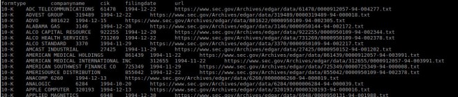
The output file will look like Figure 1 below.
Figure 1. A Linux less on all.txt.
Finally, we’ll get just the URLs for each 10-K, which we will request from the EDGAR server.
url_index = 4
outlines = []
with open("%s/all-10k-submissions.txt" % HOME_DIR, 'r') as infile:
    for line in infile:
        line = line.strip().split('\t')
        url = line[url_index]
        outlines.append(url + '\n')

with open("%s/%s" % (HOME_DIR, outfilename),'w') as outfile:
    outfile.writelines(outlines)
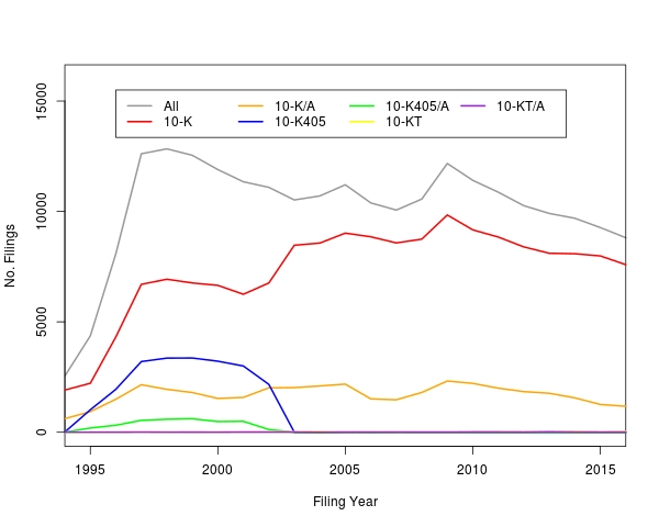
The final urls.txt file has 233,135 10-K URLs on EDGAR. In the next post I will show a method for downloading these files quickly and efficiently. Figure 2 below shows trends of the number of 10-K filed by filing year. We can see the oft cited (e.g. here, here, and here) downward trend in recent years.
Figure 2. US SEC 10-K filings by filing year, 1994-2016.
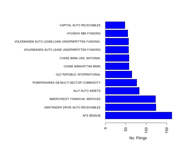
For curiosity’s sake, the top 10 10-K filers are shown in Figure 3 below.
Figure 3. Top 10 filers of US SEC 10-K filings, 1994-2016.


 . Where S, T, and E refer to the seasonal, trend, and residual (error) components, respectively.
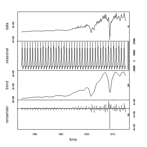


 , which makes the AR(1) process a random walk. The null and alternative hypotheses of the test are

![p,q \in [1, 5]](https://s0.wp.com/latex.php?latex=p%2Cq+%5Cin+%5B1%2C+5%5D&bg=eeeeee&fg=666666&s=0&c=20201002) . The auto.arima() function in the
. The auto.arima() function in the