Time Series Dynamics of Earnings I

In this post and the next, I build up to a VAR analysis in R–exploring the dynamics of aggregate net income, cash flow, and accruals and returns. Aggregate time series analysis is becoming very popular in accounting research. I want to provide a quick look at getting started in R on the different steps in a time series analysis on data familiar to researchers in accounting and finance.

R packages used:

• tseries
• forecast

The Data

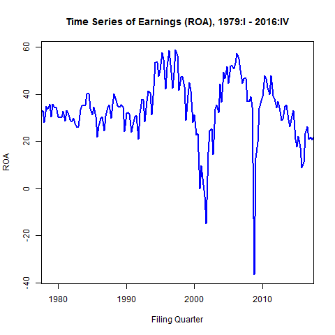
I will model raw quarterly net income (un-weighted, not scaled by, e.g., assets) from 1961 – 2017 for firms in COMPUSTAT. I’ve applied some basic filters for size, liquidity, and operating activity. For forecasting purposes, I will split the sample into training and test samples. The test sample will be the last two years (8 quarters of observations).

I decompose the trend, seasonal, and cyclical components of earnings using the stl() command. The stl() function assumes an additive series structure: . Where S, T, and E refer to the seasonal, trend, and residual (error) components, respectively.

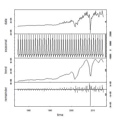
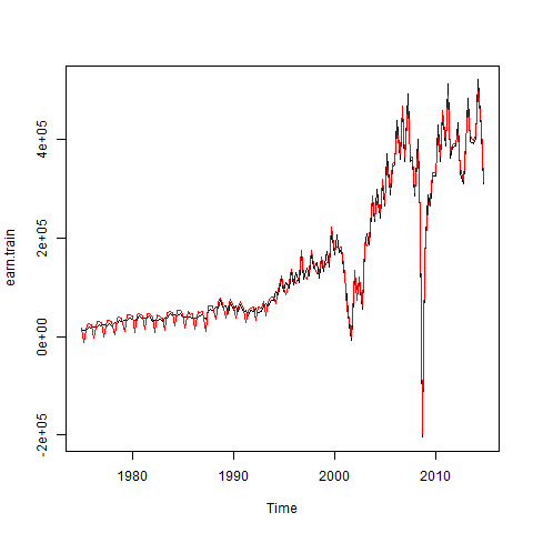
Using the seasonadj() function in forecast, I can plot the seasonally-adjusted earnings series (in red). For much of the sample period there doesn’t seem to be a significant seasonal pattern to the data. I could do a lot more to examine potential seasonality of the data, but I’ll ignore it for now.

Are Earnings Stationary?

Nonstationary time series can lead to poor inferences in modeling, specifically spurious regressions^[1] and poor forecasting performance. If variables are nonstationary we can often use a simple transformation, such as first-differencing the series or taking log transformations, to make them stationary. From the plot of aggregate earnings above, it doesn’t seem likely that earnings are stationary. As another way explore the autocovariance structure graphically I show autocorrelation and partial autocorrelation function graphs below.

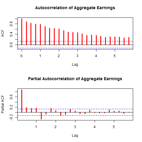
Note the slow decay in the ACF graph and the lags that are statistically significant correlates with earnings shown in the PACF. This is more evidence that the series is not stationary. Formally I perform Augmented Dickey-Fuller (ADF) tests on the series to test the null hypothesis of nonstationarity.

ADF Test

The Dickey-Fuller test for stationarity is based on an AR(1) process:

where

or, in the case of a series displaying a constant and trend

According to the Dickey-Fuller test, a time series is nonstationary when , which makes the AR(1) process a random walk. The null and alternative hypotheses of the test are

The basic AR(1) equations mentioned above are transformed, for the purpose of the DF test into

with the transformed hypothesis as

The Augmented DF test includes several lags of the variable tested. The ADF test can be of three types: with no constant and no trend, with constant and no trend, and, finally, with constant and trend. It is important to specify which DF test we want because the critical values are different for the three different types of the test. The R function adf.test() in the tseries package tests for a constant and a linear trend.^[2] Our time series is stationary if we are able to reject the null hypothesis of the ADF test.

There has been a lot of work on selecting the optimal lag length in ADF tests (see for examples ^[3] and ^[4]). In R I will investigate the tests for one to 10 lags.

k <- 10
X <- data.frame(matrix(NA, nrow = k, ncol = 2))
names(X) <- c('lags', 'p-value')
X[, 'lags'] <- 1:k
for(i in 1:k) X[i, 'p-value'] <- tseries::adf.test(earnings$roa, k = i)$p.value

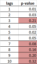
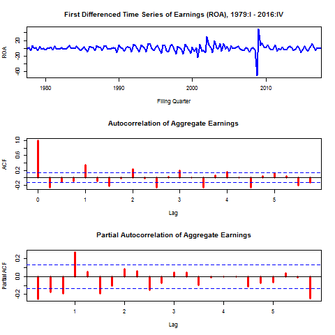
The results fail to reject the null of nonstationarity in every case, as expected. However, a simple first differencing of earnings leads to a stationary series. This implies the series is of order one integration I(1). The figures below show the time series, ACF, and PACF plots of the first-differenced earnings series. The ADF test for lags one through ten all reject the null of nonstationarity. This will be useful later for forecasting.

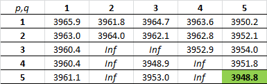
We will train a model on the differenced data. For forecasting, I’ll consider all possible ARMA(p,q) models with . The auto.arima() function in the forecast package does this nicely. The best model based on AIC is of ARMA(5,5).

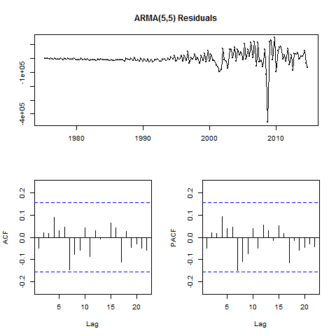
I’ll next examine the residuals of the model I’ve developed on the training data, prior to forecasting on the test data. The residuals() function combined with tsdisplay() from the forecast package will plot these diagnostics.

The figure below shows the forecast generated from this model in the last eight quarters of the sample (the hold-out sample). I’ve included error bands and superimposed the actual realizations.

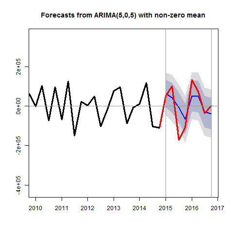
It’s important to keep in mind that what we’ve forecasted here is the change in earnings. The next step in implementing this model in a forecasting scenario might be to convert the model for the differenced earning series to one for the levels.

References:
[1] ^{Hilarious examples abound here: http://www.tylervigen.com/spurious-correlations. Most, if not all, of these correlations would go away if the series in question were first-differenced.}

[2] ^{There are various implementations of the ADF test in R, all of differing degrees of confusing, which I will cover in a future post.}

[3] ^{Ng and Perron “Unit Root Tests in ARMA Models with Data-Dependent Methods for the Selection of the Truncation Lag,” JASA, 1995.}

[4] ^{Schwert, GW “Tests for Unit Roots – A Monte-Carlo Investigation,” Journal of Business & Economic Statistics, Apr 1989. Vol 7. Issue 2. Pages 147-159.}